RNN Flip-Flop Study

Hypothesis

Biologically-inspired regularization — penalizing large synaptic weights and penalizing high neural activity — makes a small RNN more robust to noise, without needing more data or more scale.

Task and design

The 3-bit flip-flop memory task (Sussillo & Barak, 2013). Three input channels receive random +1/−1 pulses at random times; three output channels must hold the most recent sign on each channel until the next pulse flips it — 8 discrete stable memory states the network has to maintain.

Two networks with identical architecture (an RNN with 64 hidden units, plus a linear output layer) are trained and compared: Network A, a plain RNN, and Network B, the same architecture trained with an added weight-cost penalty and an activity-cost penalty. They're compared on (1) their internal dynamical structure — fixed points and attractor geometry — and (2) their robustness to injected noise.

Timeline

• Aug 23, 2026
  Stage 1 — task generator. Started; fully reset and restarted Sep 7 to use freely-random pulse signs, matching the original Sussillo & Barak formulation rather than an earlier forced-flip version.
• Sep 18, 2026
  Set up Python and VS Code from a completely bare machine — Python wasn't installed at all — then ran and verified the task generator in that environment. Stage 1 complete.
• Sep 19, 2026
  Stage 2 — Network A completed and verified.
• Sep 20, 2026
  Stage 3 — Network B first trained (20,000 iterations). Later retrained at 25,000 iterations after increasing λ_weight from 0.001 to 0.01. Complete.
• Fall 2026
  Stage 4 — fixed-point finder built and run on both networks. Stage 5 — robustness/noise testing built, debugged, and rerun across three separate runs. Both complete.
• Next
  Stage 6 — writeup complete: this page plus a final paper draft (PDF). Next: retrain from different random starts, then consider an arXiv-style submission.

Methods

• Architecture
  PyTorch nn.RNN (64 hidden units, tanh nonlinearity, batch_first) plus a linear output layer. Input and output size 3 (one per flip-flop channel), identical for both networks.
• Network A
  Trained with MSE loss and the Adam optimizer for 10,000 iterations. Verified predictions closely track the true target sign and magnitude (∼0.94–1.03) across multi-pulse sequences.
• Network B
  Same architecture, with an added weight-cost penalty (λ_weight) and activity-cost penalty (λ_activity) during training. First trained at 20,000 iterations with λ_weight = 0.001, λ_activity = 0.001. λ_weight was then increased to 0.01 (keeping λ_activity at 0.001), reasoning that synaptic weight strength is the more biologically expensive resource of the two, and retrained at 25,000 iterations — this final version converged well (task loss mostly under 0.01).

Try it — run the real experiment

This loads the actual trained weights for both networks and re-runs the noise-robustness sweep live, in your browser — a fresh random batch each time, same as the original experiment. “Raw” applies the same absolute noise to both networks (the misleading first result, below). “Scaled” corrects for each network's own hidden-state magnitude first (the fair comparison).

Finding 1 — fixed-point structure

A fixed-point finder (Sussillo & Barak style: gradient descent on a “speed” metric, ||h_t+1 − h_t||, to find hidden states where the dynamics are locally stationary) converged to genuine fixed points in both networks (final speed on the order of 1e-7 to 1e-8). Rather than 8 cleanly separated point attractors — one per memory state, as a naive picture of the task might predict — both networks showed densely packed, non-isolated fixed-point neighborhoods: over 92% of roughly 2,200 candidate points (the network's own hidden states from 20 test sequences × 110 timesteps, not random vectors) landed within 0.01 of a neighboring fixed point. This looks more like a continuous, line-attractor-like manifold. Because it appeared in both networks regardless of regularization, it's read as a structural feature of how RNNs generally solve this task, not something regularization creates or removes.

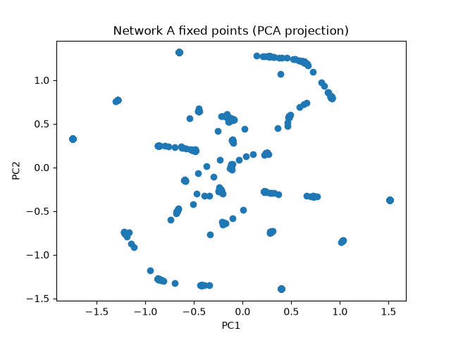
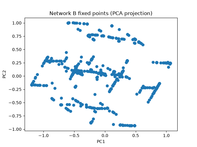
The finder itself: gradient descent on each candidate hidden state, driving it toward a point where feeding it back through the (input-free) RNN cell barely moves it, then a pairwise nearest-neighbor distance check across all candidates to see whether they land in 8 separate clusters or one dense structure. Network A's version ran 5,000 iterations of the speed minimization; Network B's ran 1,000,000 — the same script, pointed at the other network's weights, with the iteration count increased substantially and left that way rather than reconciled back to match. Both converged to the same order of final speed regardless.

import numpy as np
import torch
import torch.nn as nn


def generate_flipflop_batch(batch_size, T, n_channels=3, p=0.05):
    inputs = np.zeros((batch_size, T, n_channels))
    targets = np.zeros((batch_size, T, n_channels))

    for b in range(batch_size):
        current_state = np.zeros(n_channels)
        for t in range(T):
            for c in range(n_channels):
                if np.random.rand() < p:
                    sign = np.random.choice([-1, 1])
                    inputs[b, t, c] = sign
                    current_state[c] = sign
            targets[b, t, :] = current_state

    return inputs, targets


class NetworkB(nn.Module):
    def __init__(self, input_size=3, hidden_size=64, output_size=3):
        super().__init__()
        self.rnn = nn.RNN(input_size, hidden_size, batch_first=True)
        self.output_layer = nn.Linear(hidden_size, output_size)

    def forward(self, x):
        h_all, h_last = self.rnn(x)
        y = self.output_layer(h_all)
        return h_all, y


test_inputs_np, test_targets_np = generate_flipflop_batch(20, 110)
test_inputs = torch.tensor(test_inputs_np, dtype=torch.float32)

model = NetworkB()
model.load_state_dict(torch.load("network_a_10000iters.pth"))
model.eval()
with torch.no_grad():
    h_all, predictions = model(test_inputs)
candidates = h_all.reshape(-1, 64)
candidates = candidates.clone().detach().requires_grad_(True)
optimizer_fp = torch.optim.Adam([candidates], lr=0.01)

n_fp_iterations = 5000

for i in range(n_fp_iterations):
    zero_input = torch.zeros(candidates.shape[0], 1, 3)
    h_next, _ = model.rnn(zero_input, candidates.unsqueeze(0))
    h_next = h_next.squeeze(1)

    speed = ((h_next - candidates) ** 2).mean()

    optimizer_fp.zero_grad()
    speed.backward()
    optimizer_fp.step()

    if i % 100 == 0:
        print(i, speed.item())

candidates_detached = candidates.detach()
dist_matrix = torch.cdist(candidates_detached, candidates_detached)
dist_matrix.fill_diagonal_(float('inf'))
nearest_distances = dist_matrix.min(dim=1).values
sorted_distances = nearest_distances.sort().values
print("min:", sorted_distances.min().item())
print("max:", sorted_distances.max().item())
print("count < 0.01:", (sorted_distances < 0.01).sum().item())
print("count < 0.05:", (sorted_distances < 0.05).sum().item())
print("count < 0.1:", (sorted_distances < 0.1).sum().item())
print("count < 0.2:", (sorted_distances < 0.2).sum().item())
print("count < 0.3:", (sorted_distances < 0.3).sum().item())

import matplotlib.pyplot as plt

candidates_np = candidates_detached.numpy()
mean = candidates_np.mean(axis=0)
centered = candidates_np - mean
U, S, Vt = np.linalg.svd(centered, full_matrices=False)
projected = centered @ Vt[:2].T

plt.scatter(projected[:, 0], projected[:, 1])
plt.xlabel("PC1")
plt.ylabel("PC2")
plt.title("Network A fixed points (PCA projection)")
plt.savefig("fixed_points_pca_a.png")
plt.show()

Finding 2 — noise robustness, and a methodological trap

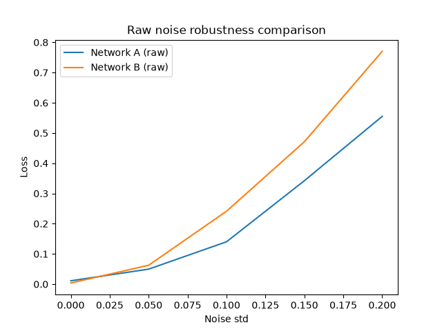
A per-timestep noisy rollout injects fresh Gaussian noise into the hidden state at every step, rather than once — a harder test, since the network never fully recovers between perturbations. Sweeping noise_std over [0, 0.05, 0.1, 0.15, 0.2]:

Raw noise (same absolute noise_std for both networks) showed Network B degrading faster than Network A as noise increased — the opposite of the hypothesis. Investigating why: Network B's activity-cost penalty gives it a meaningfully smaller typical hidden-state magnitude (∼0.12 vs. ∼0.19 for Network A). The same absolute noise is a proportionally bigger hit to Network B's smaller-scale states — the raw comparison wasn't apples-to-apples.

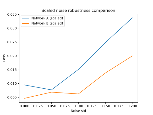
Scaled noise (noise rescaled to each network's own measured hidden-state magnitude) reversed the raw result: Network B had lower loss than Network A at every noise level. One representative run — loss_A: [0.0088, 0.0102, 0.0128, 0.0205, 0.0330], loss_B: [0.0023, 0.0048, 0.0085, 0.0129, 0.0198].

What that does and doesn't show. Network B's loss was already lower with no noise at all (0.0023 vs. 0.0088), and it was trained for 25,000 iterations to Network A's 10,000, so a lower loss at every level can come from a better baseline rather than extra robustness. Measured as loss added on top of each network's own zero-noise baseline, Network B degraded more at noise 0.05 (+0.0025 vs. +0.0014) and 0.1 (+0.0062 vs. +0.0040), and less at 0.15 (+0.0106 vs. +0.0117) and 0.2 (+0.0175 vs. +0.0242). As a ratio to its own baseline, Network B degraded more at every level (8.6× vs. 3.75× at the top level). So the scale correction clearly fixes a flaw in the raw comparison, but whether regularization makes the network more robust is not established by this pair.

Two further limits. The scaled sweep applies far less absolute noise than the raw one (about 0.02–0.04 at its top level, against 0.2), so it is a different experiment rather than the same one with a correction. And the three runs were evaluations of the same two trained networks on fresh random test batches, not three independent training runs. A rerun with matched training length, a degradation metric, and several random seeds per network is the test that would settle it.

Key findings

• 01
  Fixed-point structure is dense/continuous in both networks, not 8 discrete attractors — independent of regularization, so likely a structural feature of how small RNNs solve this task.
• 02
  Raw noise comparisons can mislead when networks operate at different internal scales. Testing both at the same absolute noise unintentionally penalizes the smaller-scale (regularized) network more.
• 03
  After correcting for scale, Network B has lower loss at every noise level — but it was already lower at zero noise, so that alone doesn't show it is more robust. The correction itself is a methodological point worth stating explicitly: robustness comparisons between networks need to control for each network's own operating scale, and for baseline loss.

Open question for the writeup

One decision isn't made yet, and it changes the outline: whether to frame the eventual paper as a small, honest methodological result — fixed points aren't discrete attractors, and robustness only shows up after correcting for scale — or to center it on the robustness finding and treat the fixed-point structure as a secondary, structural note. Both are true; which one leads changes what the paper is actually about.

How this was built

This project runs under a working agreement, set explicitly at the start: Claude explains concepts and identifies what needs figuring out; I write the actual code and debug it myself before getting anything beyond feedback on it. Two exceptions — brand-new syntax or API calls I haven't used before are taught directly, since that's vocabulary rather than logic to invent; and if I lose or corrupt a file that was already my own approved work, Claude reconstructs that exact file rather than writing new logic. The point is for this to be genuinely my own work — defensible in a college application, and eventually as a paper.

The fixed-point stage had a recurring, mundane failure mode: running or reviewing output from the wrong file — most notably a script that still pointed at Network B's saved weights while I believed it was Network A's. Each mix-up was caught by checking the torch.load(...) line or the plot title against the actual output, not by trusting what I remembered a file was called.

noisy_rollout — injecting fresh noise into the hidden state at every timestep, by looping manually rather than using the model's one-shot forward pass — was the hardest piece of code in the whole project to get right. Two of the bugs along the way were Claude's own, in code it wrote or checked, not my logic: h, _ = model.rnn(x_t, h) assigned the wrong output to the hidden state (PyTorch returns it second, not first), causing a hidden-size mismatch; and after fixing that, the output layer still carried an extra leading dimension that broke the loss computation, fixed by squeezing it out. The rest of the debugging was mine: garbled placeholder code, indentation that mixed 4- and 8-space depth, a critical bug where the function returned after only the first timestep because the stacking and return statement had drifted inside the loop, and swapped variable names between the two networks. None of it was the underlying logic being wrong — it was the normal, tedious mechanics of learning to write real code by hand.

Rough edges along the way

For my own awareness more than anything else — not a complaint about the process, just what actually slowed things down:

• Setup
  Python wasn't installed at all before Stage 1 was finished — installed from scratch via the python.org installer, added to PATH, numpy via pip.
• File identity
  Files kept getting auto-named after their first line of code rather than something meaningful (a few still sit in the repository this way). More than once I reviewed output from a different file than I thought I was running — fixed by checking what a file actually loads, not the filename in memory.
• Mechanics over logic
  Indentation depth, stray characters, and non-Python keywords slipping in were the single biggest source of back-and-forth — not because the design work was wrong, but because small mechanical slips kept breaking otherwise-correct code.

Noise-robustness code

The analysis script for Stages 3–5 — loading the trained weights, running the robustness experiments, producing the comparison plots — shown exactly as it exists in the repository. (One harmless quirk left as-is: the matplotlib import ended up inside the last loop rather than at the top; it just re-imports every iteration.) The fixed-point finder that produced the Finding 1 plots is shown above, in that section; the task generator and the two training loops (Stages 1–3) were written and verified in earlier sessions and aren't reproduced here.

The exact trained weights the demo above uses are the same ones loaded here — exported from the two .pth files to JSON, viewable directly at /data/rnn-weights.json.

import numpy as np
import torch
import torch.nn as nn


def generate_flipflop_batch(batch_size, T, n_channels=3, p=0.05):
    inputs = np.zeros((batch_size, T, n_channels))
    targets = np.zeros((batch_size, T, n_channels))

    for b in range(batch_size):
        current_state = np.zeros(n_channels)
        for t in range(T):
            for c in range(n_channels):
                if np.random.rand() < p:
                    sign = np.random.choice([-1, 1])
                    inputs[b, t, c] = sign
                    current_state[c] = sign
            targets[b, t, :] = current_state

    return inputs, targets


class NetworkB(nn.Module):
    def __init__(self, input_size=3, hidden_size=64, output_size=3):
        super().__init__()
        self.rnn = nn.RNN(input_size, hidden_size, batch_first=True)
        self.output_layer = nn.Linear(hidden_size, output_size)

    def forward(self, x):
        h_all, h_last = self.rnn(x)
        y = self.output_layer(h_all)
        return h_all, y


def noisy_rollout(model, x, noise_std):
    batch_size = x.shape[0]
    T = x.shape[1]
    hidden_size = 64
    h = torch.zeros(1, batch_size, hidden_size)
    outputs = []
    for t in range(T):
        x_t = x[:, t:t+1, :]
        _, h = model.rnn(x_t, h)
        noise = torch.randn_like(h) * noise_std
        h = h + noise
        y_t = model.output_layer(h.squeeze(0))
        outputs.append(y_t)
    predictions = torch.stack(outputs, dim=1)
    return predictions


model_a = NetworkB()
model_a.load_state_dict(torch.load("network_a_10000iters.pth"))
model_a.eval()

model_b = NetworkB()
model_b.load_state_dict(torch.load("network_b_25000iters_lw0.01_la0.001.pth"))
model_b.eval()


loss_fn = nn.MSELoss()
noise_levels = [0, 0.05, 0.1, 0.15, 0.2]

losses_a = []
for noise_std in noise_levels:
    inputs_np, targets_np = generate_flipflop_batch(64, 110)
    inputs = torch.tensor(inputs_np, dtype=torch.float32)
    targets = torch.tensor(targets_np, dtype=torch.float32)
    predictions = noisy_rollout(model_a, inputs, noise_std)
    loss = loss_fn(predictions, targets)
    losses_a.append(loss.item())
    print(noise_std, loss.item())

losses_b = []
for noise_std in noise_levels:
    inputs_np, targets_np = generate_flipflop_batch(64, 110)
    inputs = torch.tensor(inputs_np, dtype=torch.float32)
    targets = torch.tensor(targets_np, dtype=torch.float32)
    predictions = noisy_rollout(model_b, inputs, noise_std)
    loss = loss_fn(predictions, targets)
    losses_b.append(loss.item())
    print(noise_std, loss.item())

test_inputs_np, test_targets_np = generate_flipflop_batch(20, 110)
test_inputs = torch.tensor(test_inputs_np, dtype=torch.float32)
with torch.no_grad():
    h_all_a, predictions_a = model_a(test_inputs)
print("Network A magnitude:", h_all_a.abs().mean())
with torch.no_grad():
    h_all_b, predictions_b = model_b(test_inputs)
print("Network B magnitude:", h_all_b.abs().mean())

losses_a_scaled = []
for noise_std in noise_levels:
    inputs_np, targets_np = generate_flipflop_batch(64, 110)
    inputs = torch.tensor(inputs_np, dtype=torch.float32)
    targets = torch.tensor(targets_np, dtype=torch.float32)
    scaled_noise = h_all_a.abs().mean().item() * noise_std
    predictions = noisy_rollout(model_a, inputs, scaled_noise)
    loss = loss_fn(predictions, targets)
    losses_a_scaled.append(loss.item())
    print(noise_std, loss.item())

losses_b_scaled = []
for noise_std in noise_levels:
    inputs_np, targets_np = generate_flipflop_batch(64, 110)
    inputs = torch.tensor(inputs_np, dtype=torch.float32)
    targets = torch.tensor(targets_np, dtype=torch.float32)
    scaled_noise = h_all_b.abs().mean().item() * noise_std
    predictions = noisy_rollout(model_b, inputs, scaled_noise)
    loss = loss_fn(predictions, targets)
    losses_b_scaled.append(loss.item())
    print(noise_std, loss.item())
    import matplotlib.pyplot as plt

plt.plot(noise_levels, losses_a, label="Network A (raw)")
plt.plot(noise_levels, losses_b, label="Network B (raw)")
plt.xlabel("Noise std")
plt.ylabel("Loss")
plt.title("Raw noise robustness comparison")
plt.legend()
plt.savefig("robustness_raw.png")
plt.show()

plt.plot(noise_levels, losses_a_scaled, label="Network A (scaled)")
plt.plot(noise_levels, losses_b_scaled, label="Network B (scaled)")
plt.xlabel("Noise std")
plt.ylabel("Loss")
plt.title("Scaled noise robustness comparison")
plt.legend()
plt.savefig("robustness_scaled.png")
plt.show()

Paper draft

The write-up of the project above, in a more formal register. It's still a draft — a small, single-pair pilot, not a finished paper. Two spots on this page have been revised from the downloadable PDF (marked inline, below): the framing of the Introduction, and a precision fix to what the Results section's “three runs” claim actually covers. The PDF at the end is the final draft as written, without those two revisions.

Connection to “How I Define AGI”

This project is a hands-on test of the argument in How I Define AGI (a follow-up to an earlier essay, “My Perception of AGI”): that AGI is more likely to come from studying the brain's architecture and efficiency than from scaling alone. The essay was deliberately written in a more professional register than the earlier, more conversational essay, after working through the CBMM (Center for Brains, Minds and Machines) lecture series — with this project as the intended next step: putting that thesis to an actual, concrete test rather than leaving it as argument alone.

Status and next step

Stages 1–5 (task generator, both networks, the fixed-point finder, and the robustness experiments) and the writeup (Stage 6) are complete. The paper is a final draft of a small pilot: one trained pair of networks, one task. Next: retrain both networks from different random starting points, with matched training length, to see whether the lower loss reflects real robustness or just a better baseline; decide the open framing question above, and then consider a short arXiv-style submission.

References

Sussillo, D., & Barak, O. (2013). Opening the Black Box: Low-Dimensional Dynamics in High-Dimensional Recurrent Neural Networks. Neural Computation, 25(3), 626–649. https://doi.org/10.1162/NECO_a_00409